Homework 5
Luis Acosta
library(tidyverse)## -- Attaching packages ----------------------------------------------------------------- tidyverse 1.2.1 --## v tibble 1.3.4 v purrr 0.2.4
## v tidyr 0.7.2 v dplyr 0.7.4
## v readr 1.1.1 v stringr 1.2.0
## v tibble 1.3.4 v forcats 0.2.0## -- Conflicts -------------------------------------------------------------------- tidyverse_conflicts() --
## x stringr::boundary() masks strucchange::boundary()
## x dplyr::combine() masks randomForest::combine()
## x dplyr::filter() masks stats::filter()
## x dplyr::lag() masks stats::lag()
## x purrr::lift() masks caret::lift()
## x randomForest::margin() masks ggplot2::margin()
## x dplyr::select() masks MASS::select()
## x dplyr::slice() masks xgboost::slice()hwlink <- "https://raw.githubusercontent.com/reisanar/datasets/master/clusterThis.csv"
hwdata <- read_csv(hwlink)## Parsed with column specification:
## cols(
## x = col_double(),
## y = col_double()
## )Problem 1 : K-means
ggplot(hwdata, aes(x=x,y=y)) + geom_point()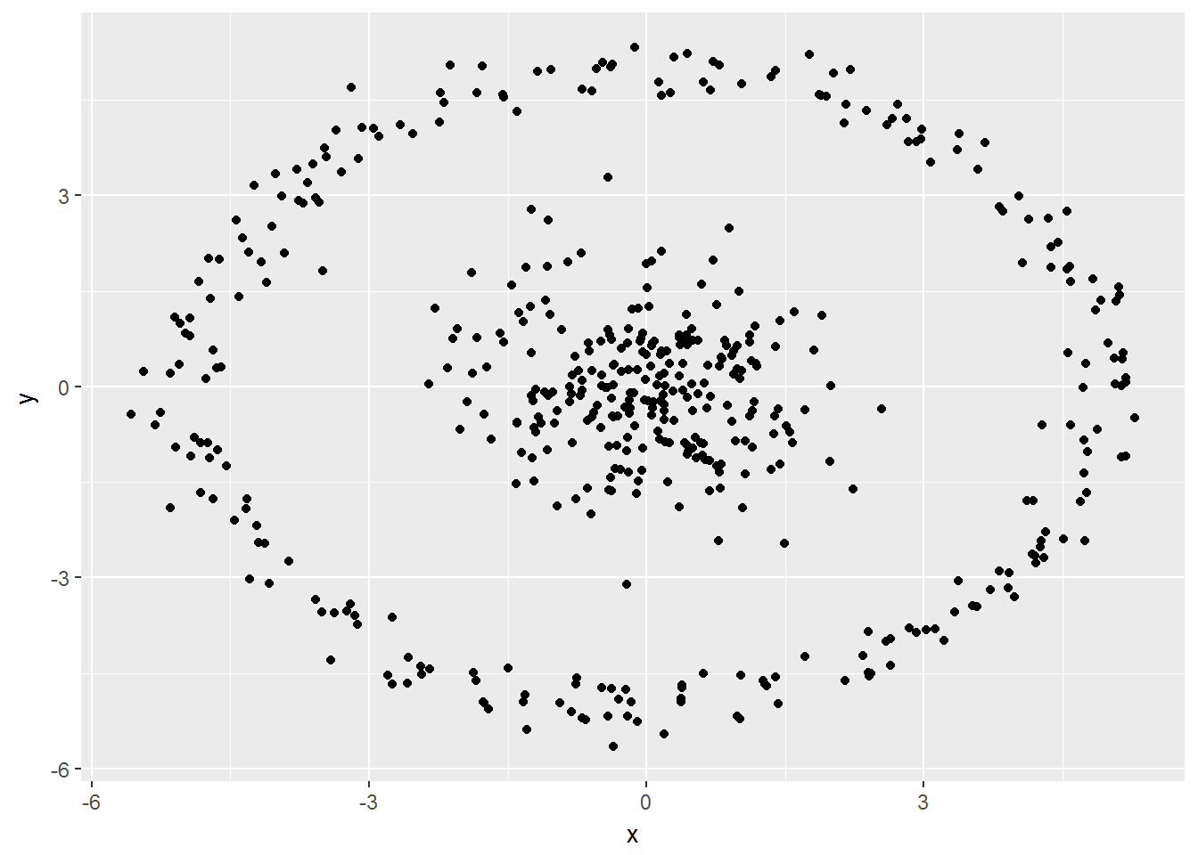 - Do you see any type of clusters/groups right away?
2 groups
- Use k-means to try to find two (2) clusters in this dataset. Use the base R function kmeans():
km_clusterThis <- kmeans(hwdata[, c("y", "x")], centers = 2)str(km_clusterThis)## List of 9
## $ cluster : int [1:500] 2 2 2 2 2 1 2 1 2 2 ...
## $ centers : num [1:2, 1:2] -2.278 1.332 1.298 -0.831
## ..- attr(*, "dimnames")=List of 2
## .. ..$ : chr [1:2] "1" "2"
## .. ..$ : chr [1:2] "y" "x"
## $ totss : num 6676
## $ withinss : num [1:2] 1875 2712
## $ tot.withinss: num 4587
## $ betweenss : num 2089
## $ size : int [1:2] 195 305
## $ iter : int 1
## $ ifault : int 0
## - attr(*, "class")= chr "kmeans"- Plot the points again colored by the associated cluster found in the previous step
km_results <- as.factor(km_clusterThis$cluster)ggplot(hwdata, aes(x=x,y=y, color = km_results)) + geom_point()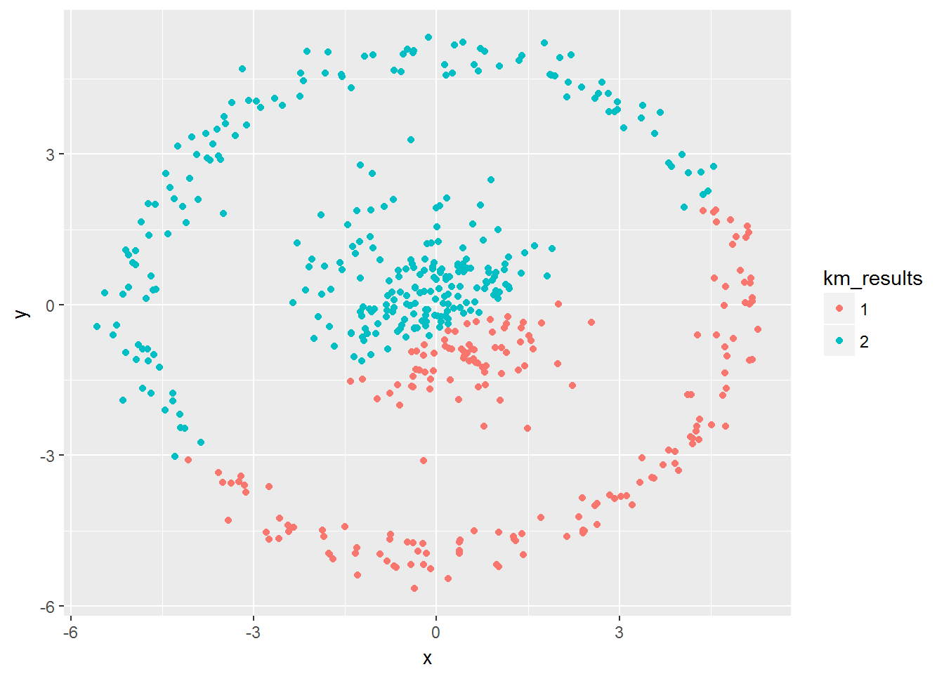
Problem 2: Hierarchical clustering
- Use hierarchical clustering (with a single linkage) to try to find the groups in this dataset. You can use the hclust() function from base R.
dis <- dist(hwdata[, c("x", "y")])
hc_hwdata <- hclust(dis, method = "single")str(hc_hwdata)## List of 7
## $ merge : int [1:499, 1:2] -113 -295 -83 -159 -64 -261 -371 -68 -193 -65 ...
## $ height : num [1:499] 0.0132 0.0134 0.0176 0.0197 0.0197 ...
## $ order : int [1:500] 277 444 279 483 293 473 362 391 460 478 ...
## $ labels : NULL
## $ method : chr "single"
## $ call : language hclust(d = dis, method = "single")
## $ dist.method: chr "euclidean"
## - attr(*, "class")= chr "hclust"- Cut the dendrogram tree to 2 clusters using the cutree() function
cut2 <- cutree(hc_hwdata, 2)hc_result <- as.factor(cut2)- Plot the points with this new cluster assignment:
ggplot(hwdata, aes(x=x,y=y, color = hc_result)) + geom_point()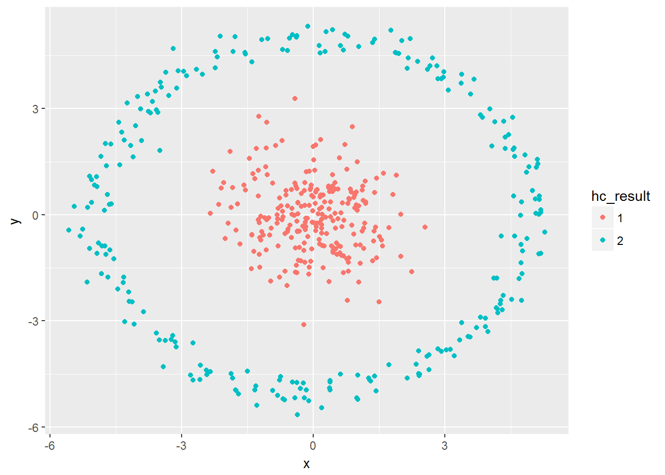
Problem 2: Data Transformation
- We can use a transformation on the data set to help with the clustering problem. For example, transforming the data into polar coordinates,might be a good idea in this case.
polar <- hwdata %>% transform(r = sqrt(x^2 + y^2), theta=atan(y/x))km_polar <- kmeans(polar[, c("r", "theta")], centers = 2)- Plot the points again with this new assignment of clusters:
str(km_polar)## List of 9
## $ cluster : int [1:500] 2 2 2 2 2 2 2 2 2 2 ...
## $ centers : num [1:2, 1:2] 4.95508 1.1842 0.03064 -0.00852
## ..- attr(*, "dimnames")=List of 2
## .. ..$ : chr [1:2] "1" "2"
## .. ..$ : chr [1:2] "r" "theta"
## $ totss : num 2324
## $ withinss : num [1:2] 241 306
## $ tot.withinss: num 547
## $ betweenss : num 1777
## $ size : int [1:2] 253 247
## $ iter : int 1
## $ ifault : int 0
## - attr(*, "class")= chr "kmeans"km_results2 <- as.factor(km_polar$cluster)ggplot(polar, aes(x=r,y=theta, color = km_results2)) + geom_point()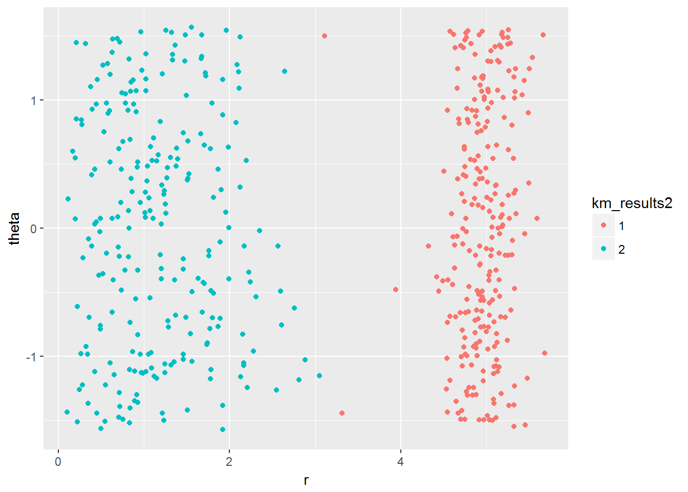
- Is this a better cluster assignment with k-means than from problem 1?
I think the transformation performs an improved separation of clusters. In problem number 1, groups are very close at some points and in this case, we can identify clearly two groups. In case the groups are customers, a marketing campaign can give us better results.